Rejection Sampling
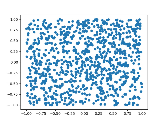
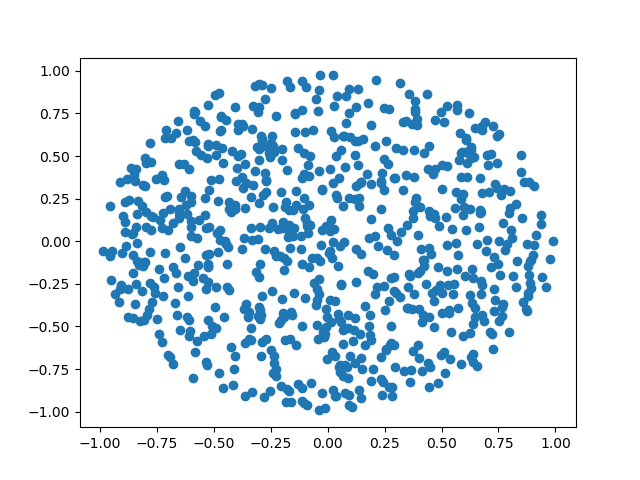
Sometimes we want to sample from a distribution that we don’t necessarily know how to sample from directly (i.e. it isn’t one of the distributions that comes built-in to our favorite software package). The classic example is generating random points uniformly distributed within a circle. The idea is to enclose the circle within a square. It is easy to generate uniform points inside of a square. We do that, and then throw away all points that don’t fall inside the circle. Here is some python code that does this:
import numpy as np
import matplotlib.pyplot as plt


def square_uniform_sampling(num_samples):
    return np.random.uniform(low=[-1,-1], high=[1,1], size=(num_samples,2))


def point_in_circle(point):
    return point[0]**2 + point[1]**2 < 1


def get_points_in_circle(points):
    return points[list(map(point_in_circle, points))]


def circle_uniform_sampling(num_samples):
    square_points = square_uniform_sampling(num_samples)
    return get_points_in_circle(square_points)


def plot(data):
    plt.scatter(data[:,0], data[:,1])
    plt.show()


def main():
    num_samples = 1000
    square_samples = square_uniform_sampling(num_samples)
    plot(square_samples)
    circle_samples = circle_uniform_sampling(num_samples)
    plot(circle_samples)
This script generates the following plots
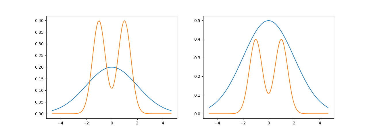
The example above is a particular case of rejection sampling where we are using a uniform distribution as our proposal distribution. In general, we aren’t limited to using a uniform distribution as a proposal (in fact, our sampling will be more efficient when we use a proposal distribution that more closely approximates the distribution we actually want to sample from). It is necessary that our proposal distribution also “envelopes” the distribution we care about as seen in the figure (the left plot has the two densities, while the right plot has the proposal density multiplied by some constant \(M\) so that it is above the other density everywhere).
Why do we need to envelope the distribution of interest? Well, if we could sample uniformly from the region below the density function of interest we would be done because this is the same as sampling from the density function itself.
Informally, the algorithm samples a point from some distribution and then decides whether to accept or reject (hence rejection sampling) according to some rule.
Let \(p\) be the distribution of interest and \(q\) be the propsal distribution. The rejection sampling algorithm is as follows
- Sample from the proposal distribution, \(x \sim q(x)\)
- Sample from a uniform distribution \(u \sim U(0,1)\)
- If \(u < \frac{p(x)}{M q(x)}\) then accept \(x\), otherwise reject \(x\).
The intuition for why this works is that for a fixed \(x\) only accept according to the ratio of \(p\) and \(q\) which corrects for the areas that we are oversampling due to the envelope principle.
It is important to note that rejection sampling is very inefficient in high-dimensional spaces because the acceptance probability will almost always be very small. Here is some code implementing rejection sampling for a Gaussian mixture model using a Gaussian distribution as the proposal distribution (the two densities shown above are the densities used in this example):
import numpy as np
import matplotlib.pyplot as plt
import scipy.stats
import seaborn as sns


def two_component_mixture_pdf(x):
    return (scipy.stats.norm.pdf(x, loc=-1, scale=0.5) + scipy.stats.norm.pdf(x, loc=1, scale=0.5))/2


def proposal_pdf(x):
    return scipy.stats.norm.pdf(x, loc=0, scale=2)


def two_component_mixture(num_samples, mixture_proportion=0.5):
    # generate mixture distribution
    component1_proportion = mixture_proportion
    component2_proportion = 1 - component1_proportion

    component1 = scipy.stats.norm.rvs(loc=-1, scale=0.5, size=int(num_samples * component1_proportion))
    component2 = scipy.stats.norm.rvs(loc=1, scale=0.5, size=int(num_samples * component2_proportion))

    data = np.append(component1, component2)
    return data


def sample_from_proposal():
    return scipy.stats.norm.rvs(loc=0, scale=2)


def rejection_sampling(num_samples, density_of_interest, proposal_density, envelope_constant):
    data = []
    i = 0
    while i != num_samples:
        x = sample_from_proposal()
        u = scipy.stats.uniform.rvs()

        if u < density_of_interest(x) / (envelope_constant * proposal_density(x)):
            data.append(x)
            i += 1

    return np.array(data)


def main():
    num_samples = 10000
    direct_samples = two_component_mixture(num_samples)

    # envelope constant was found by inspection of plots and is not optimal
    envelope_constant = 2.5

    data = rejection_sampling(num_samples, two_component_mixture_pdf, proposal_pdf, 2.5)
    sns.distplot(direct_samples)
    plt.show()
    sns.distplot(data)
    plt.show()
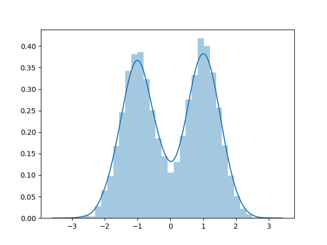
Here is a dataset sampled using rejection sampling:
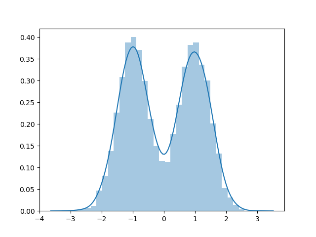
Here is a dataset sampled directly:
Adaptive rejection sampling
So what is adaptive rejection sampling? It is an extension of the method that tries to be clever about how we bound our density of interest. As I said earlier, if the proposal density is closer to the density of interest we will be more efficient in our rejection sampling (by rejecting fewer points). Adaptive rejection sampling only works in the case where the density of interest is log-concave. It involves starting with a piecewise linear density function as your envelope. Then, with each rejected sample, you improve the piecewise approximation of the proposal distribution.
This method involves some tedious bookkeeping and computing the intersection of hyperplanes.
Adaptive Rejection Metropolis Sampling (ARMS)
There is no reason that this idea of adapting a proposal distribution is limited to rejection sampling. It can also be used to improve the convergence of Metropolis sampling. There are several papers in the citations of the Rejection sampling Wikipedia page that develop this idea.
Ziggurat algorithm
Another cool variation of rejection sampling is the Ziggurat algorithm. The Wikipedia page has a really nice animation of the idea.