Imagine that your computer is only able to sample from a uniform distribution on \([0,1]\). This is useful, but often you want to sample from a distribution other than uniform (for example, normal, binomial, Poisson, etc.). Is there a way to make your uniform random variable look like different distributions? For univariate distributions inverse transform sampling provides a solution to this problem.

The key insight is to notice that if \(X\) is a continuous random variable with cdf \(F_X\), then \(F_X\) is distributed uniformly on \([0,1]\). Armed with this fact, we can simulate draws of \(X\) using draws from a uniform distribution and \(F_X^{-1}\).

The CDF has a uniform distribution

Let’s prove the fact that \(F_X\) is distributed uniformly on \([0,1]\). We’ll assume that \(F_X\) is strictly increasing so that we don’t have to worry about how we define its inverse (if you don’t make this assumption you can define \(F^{-1}(y) = \inf \{x : F(x) \geq y\}\)). This assumption means that \(F_X^{-1}\) is well-defined. Let \(Y = F_X(x)\). Consider

and since we have an inverse

Notice that this is exactly the cdf of a uniform distribution and so \(Y = F_X(x)\) is distributed uniformly.

Correctness of inverse transform sampling

The idea of inverse transform sampling is to sample a uniform random variable and use the inverse cdf of the distribution we care about to change the distribution of our samples. Let’s prove that this procedure works. Let \(U\) be a uniform random variable and let \(F\) be a strictly increasing cdf for the distribution that we care about. The claim is that \(F^{-1}(U)\) has \(F\) as its cdf. Consider

and since \(U\) is uniform its cdf is simply

and this is what we wanted to prove. This means that this simple procedure works in principle (although there may be computational considerations for practical use).

Inverse cdf

What I’ve been calling the inverse cdf is actually called the quantile function. Let’s do one easy example. The exponential distribution (with parameter \(\lambda\) has cdf

for all \(x \geq 0\). It is straightforward (using algebra) to show that

Example of inverse transform sampling

The following code shows inverse transform sampling in action for the exponential distribution. First, we import the Python modules we need

import matplotlib.pyplot as plt
import numpy as np

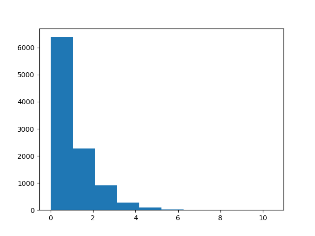
Next, lets sample from an exponential distribution (with parameter 1) and take a look at what the histogram looks like.

n = 10000
exponential_samples = np.random.exponential(1,n)
plt.hist(exponential_samples)
plt.show()

Here is what the exponential distribution looks like when we sample from it directly using NumPy.

Next, we define the quantile function for the exponential distribution.

def quantile_exponential_distribution(lambda_param, y):
    return -np.log(1-y) / lambda_param

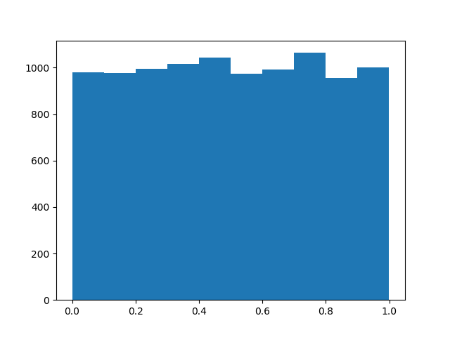
In order to use inverse transform sampling, we need to sample from a normal distribution, which we can do easily using NumPy.

uniform_samples = np.random.uniform(0,1,n)
plt.hist(uniform_samples)
plt.show()

Here is what the uniform distribution looks like when we sample from it using NumPy.

Finally, we can transform the uniform samples using our quantile function to obtain exponential samples.

transformed_exponential_samples = quantile_exponential_distribution(lambda_param=1, y=uniform_samples)
plt.hist(transformed_exponential_samples)
plt.show()

Here is what the transformed distribution looks like.

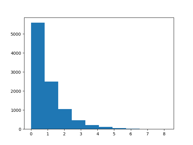
This is exactly what the exponential distribution looks like.

Computational considerations

One challenge is that to generate a large number of samples from a distribution, you must compute the quantile function many times. According to Wikipedia: “one possible way to reduce the number of inversions while obtaining a large number of samples is the application of the so-called Stochastic Collocation Monte Carlo sampler (SCMC sampler) within a polynomial chaos expansion framework. This allows us to generate any number of Monte Carlo samples with only a few inversions of the original distribution with independent samples of a variable for which the inversions are analytically available, for example the standard normal variable.”

I’m not familiar with SCMC, but they cite a paper The stochastic collocation Monte Carlo sampler: Highly efficient sampling from “expensive” distributions by Grzelak et al.. Maybe I’ll read the paper and write a follow up post.